25 Model comparisons

25.1 Objectives

Questions

• How do I compare linear models?
• How do decide which one is the “best” model?

Objectives

• Be able to compare models using the Akaike Information Criterion (AIC)
• Use AIC in the context of Backwards Stepwise Elimination in R

25.2 Purpose and aim

In the previous example we used a single dataset and fitted five linear models to it depending on which predictor variables we used. Whilst this was fun (seriously, what else would you be doing right now?) it seems that there should be a “better way”. Well, thankfully there is! In fact there a several methods that can be used to compare different models in order to help identify “the best” model. More specifically, we can determine if a full model (which uses all available predictor variables and interactions) is necessary to appropriately describe the dependent variable, or whether we can throw away some of the terms (e.g. an interaction term) because they don’t offer any useful predictive power.

Here we will use the Akaike Information Criterion in order to compare different models.

25.3 Section commands

New commands in this section:

Function	Description
extractAIC()	Extract the Akaike Information Criterion from a fitted model
step()	Performs backwards stepwise elimination on a model

25.4 Data and hypotheses

This section uses the data/tidy/CS5-Ladybird.csv data set. This data set comprises of 20 observations of three variables (one dependent and two predictor). This records the clutch size (eggs) in a species of ladybird alongside two potential predictor variables; the mass of the female (weight), and the colour of the male (male) which is a categorical variable.

25.5 Backwards Stepwise Elimination

First, load the data and store it in an object called ladybird. Then visualise the data.

ladybird <- read_csv("data/tidy/CS5-Ladybird.csv")

# visualise the data
ladybird %>% 
  ggplot(aes(x = weight, y = eggs,
             colour = male)) +
  geom_point() +
  scale_color_brewer(palette = "Dark2")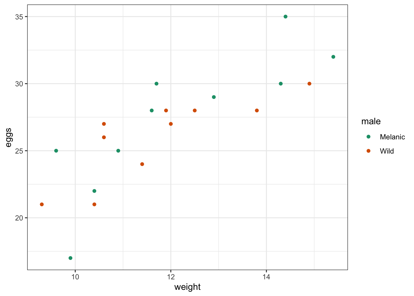

25.5.1 Comparing models with AIC (step 1)

First, we construct the full linear model:

# define the full model
lm_full <- lm(eggs ~ weight * male,
              data = ladybird)

# view the model summary
summary(lm_full)

Now we construct a reduced model (i.e. the next simplest model) which doesn’t have interactions:

# define the model
lm_red <- lm(eggs ~ weight + male,
             data = ladybird)

# view the model summary
summary(lm_red)

To compare the two models we simply use the command extractAIC() on each model.

extractAIC(lm_full)

## [1]  4.00000 41.28452

extractAIC(lm_red)

## [1]  3.00000 40.43819

For each line the first number tells you how many parameters are in your model and the second number tells you the AIC score for that model. Here we can see that the full model has 4 parameters (the intercept, the coefficient for the continuous variable weight, the coefficient for the categorical variable male and a coefficient for the interaction term weight:male) and an AIC score of 41.3 (1dp). The reduced model has a lower AIC score of 40.4 (1dp) with only 3 parameters (since we’ve dropped the interaction term). There are different ways of interpreting AIC scores but the most widely used interpretation says that:

• if the difference between two AIC scores is greater than 2 then the model with the smallest AIC score is more supported than the model with the higher AIC score
• if the difference between the two models’ AIC scores is less than 2 then both models are equally well supported

This choice of language (supported vs significant) is deliberate and there are areas of statistics where AIC scores are used differently from the way we are going to use them here (ask if you want a bit of philosophical ramble from me). However, in this situation we will use the AIC scores to decide whether our reduced model is at least as good as the full model. Here since the difference in AIC scores is less than 2, we can say that dropping the interaction term has left us with a model that is both simpler (fewer terms) and as least as good (AIC score) as the full model. As such our reduced model eggs ~ weight + male is designated our current working minimal model.

25.5.2 Comparing models with AIC (step 2)

Next, we see which of the remaining terms can be dropped. We will look at the models where we have dropped both male and weight (i.e. eggs ~ weight and eggs ~ male) and compare their AIC values with the AIC of our current minimal model (eggs ~ weight + male). If the AIC values of at least one of our new reduced models is lower (or at least no more than 2 greater) than the AIC of our current minimal model, then we can drop the relevant term and get ourselves a new minimal model. If we find ourselves in a situation where we can drop more than one term we will drop the term that gives us the model with the lowest AIC.

Drop the variable weight and examine the AIC:

# define the model
lm_male <- lm(eggs ~ male,
              data = ladybird)

# extract the AIC
extractAIC(lm_male)

## [1]  2.00000 59.95172

Drop the variable male and examine the AIC:

# define the model
lm_weight <- lm(eggs ~ weight,
                data = ladybird)

# extract the AIC
extractAIC(lm_weight)

## [1]  2.00000 38.76847

Considering both outputs together and comparing with the AIC of our current minimal model (40.4) we can see that dropping male has decreased the AIC further to 38.8, whereas dropping weight has actually increased the AIC to 60.0 and thus worsened the model quality.

Hence we can drop male and our new minimal model is eggs ~ weight.

25.5.3 Comparing models with AIC (step 3)

Our final comparison is to drop the variable weight and compare this simple model with a null model (eggs ~ 1), which assumes that the brood size is constant across all parameters.

Drop the variable weight and see if that has an effect:

# define the model
lm_null <- lm(eggs ~ 1,
              data = ladybird)

# extract the AIC
extractAIC(lm_null)

## [1]  1.00000 58.46029

The AIC of our null model is quite a bit larger than that of our current minimal model eggs ~ weight and so we conclude that weight is important. As such our minimal model is eggs ~ weight.

So, in summary, we could conclude that:

Female size is a useful predictor of clutch size, but male type is not so important.

At this stage we can analyse the minimal linear (lm.weight) model using the anova() function, and we should consider the diagnostic plots by using the plot(lm.weight) command.

25.6 Notes on Backwards Stepwise Elimination

This method of finding a minimal model by starting with a full model and removing variables is called backward stepwise elimination. Although regularly practised in data analysis, there is increasing criticism of this approach, with calls for it to be avoided entirely.

Why have we made you work through this procedure then? Given their prevalence in academic papers, it is very useful to be aware of these procedures and to know that there are issues with them. In other situations, using AIC for model comparisons are justified and you will come across them regularly. Additionally, there may be situations where you feel there are good reasons to drop a parameter from your model – using this technique you can justify that this doesn’t affect the model fit. Taken together, using backwards stepwise elimination for model comparison is still a useful technique.

Performing backwards stepwise elimination manually can be quite tedious. Thankfully R acknowledges this and there is a single inbuilt function called step() that can perform all of the necessary steps for you using AIC.

## Start:  AIC=41.28
## eggs ~ weight * male
## 
##               Df Sum of Sq    RSS    AIC
## - weight:male  1    6.2724 111.90 40.438
## <none>                     105.63 41.285
## 
## Step:  AIC=40.44
## eggs ~ weight + male
## 
##          Df Sum of Sq    RSS    AIC
## - male    1     1.863 113.77 38.768
## <none>                111.90 40.438
## - weight  1   216.196 328.10 59.952
## 
## Step:  AIC=38.77
## eggs ~ weight
## 
##          Df Sum of Sq    RSS    AIC
## <none>                113.77 38.768
## - weight  1    222.78 336.55 58.460

## 
## Call:
## lm(formula = eggs ~ weight, data = ladybird)
## 
## Coefficients:
## (Intercept)       weight  
##       4.320        1.873

This will perform a full backwards stepwise elimination process and will find the minimal model for you. The output should be familiar to you but ask a demonstrator if you have any questions.

Yes, I could have told you this earlier, but where’s the fun in that? (it is also useful for you to understand the steps behind the technique I suppose…)

25.7 Exercise: BSE

Exercise 25.1 BSE on trees and airpoll

Use the internal dataset trees and the airpoll dataset from earlier.

• Perform a backwards stepwise elimination on both of these datasets and discover the minimal model using AIC.

NB: if an interaction term is significant then any main factor that is part of the interaction term cannot be dropped from the model.

• If you’re feeling up for it attempt a backwards stepwise elimination process on the internal CO2 dataset. This data frame has 1 dependent variable (uptake) and 4 predictor variables (Plant, Type, Treatment, conc). Unfortunately, the dataset does not contain enough data to construct a full linear model using all 4 predictor variables (with all of the interactions), so ignore the Plant variable and take uptake ~ Type + Treatment + conc + Type:Treatment + Type:conc + Treatment:conc + Type:Treatment:conc as your full model.

Answer

This is relatively straightforward using the step() function.

We need to first construct the full linear model and then simply pass this linear model object to the step function and R does the rest.

25.7.1 trees dataset

We construct a full linear model with both Height, Girth and the interaction between them and then we run the step() function:

# define the full model
lm_trees <- lm(Volume ~ Girth * Height,
               data = trees)

# perform BSE
step(lm_trees)

## Start:  AIC=65.49
## Volume ~ Girth * Height
## 
##                Df Sum of Sq    RSS    AIC
## <none>                      198.08 65.495
## - Girth:Height  1    223.84 421.92 86.936

## 
## Call:
## lm(formula = Volume ~ Girth * Height, data = trees)
## 
## Coefficients:
##  (Intercept)         Girth        Height  Girth:Height  
##      69.3963       -5.8558       -1.2971        0.1347

This BSE approach only gets as far as the first step (trying to drop the interaction term). We see immediately that dropping the interaction term makes the model worse and so the process stops. On the next line (underneath Call:) we see that the best model is still the full model and then we get to see the coefficients for each term.

25.7.2 airpoll dataset

## Rows: 16 Columns: 4
## ── Column specification ────────────────────────────────────────────────────────
## Delimiter: ","
## chr (1): treatment_plant
## dbl (3): id, daily_temp, hydrogen_sulfide
## 
## ℹ Use `spec()` to retrieve the full column specification for this data.
## ℹ Specify the column types or set `show_col_types = FALSE` to quiet this message.

We construct a full linear model with both treatment_plant, daily_temp and the interaction between them and then we run the step function:

# define the full model
lm_airpoll <- lm(hydrogen_sulfide ~ treatment_plant * daily_temp,
                 data = airpoll)

# perform BSE
step(lm_airpoll)

## Start:  AIC=-19.04
## hydrogen_sulfide ~ treatment_plant * daily_temp
## 
##                              Df Sum of Sq    RSS     AIC
## <none>                                    2.9520 -19.041
## - treatment_plant:daily_temp  1     1.447 4.3991 -14.659

## 
## Call:
## lm(formula = hydrogen_sulfide ~ treatment_plant * daily_temp, 
##     data = airpoll)
## 
## Coefficients:
##                 (Intercept)             treatment_plantB  
##                     6.20495                     -2.73075  
##                  daily_temp  treatment_plantB:daily_temp  
##                    -0.05448                      0.18141

Again, this BSE approach only gets as far as the first step (trying to drop the interaction term). We see immediately that dropping the interaction term makes the model worse and so the process stops. On the next line (underneath Call:) we see that the best model is still the full model and then we get to see the coefficients for each term.

25.7.3 CO2 dataset

# define the model, ignore the Plant variable
lm_co2 <- lm(uptake ~ Type + Treatment + conc
             + Type:Treatment + Type:conc + Treatment:conc
             + Type:Treatment:conc,
             data = CO2)
step(lm_co2)

## Start:  AIC=302.6
## uptake ~ Type + Treatment + conc + Type:Treatment + Type:conc + 
##     Treatment:conc + Type:Treatment:conc
## 
##                       Df Sum of Sq    RSS    AIC
## - Type:Treatment:conc  1    55.535 2602.7 302.41
## <none>                             2547.2 302.60
## 
## Step:  AIC=302.41
## uptake ~ Type + Treatment + conc + Type:Treatment + Type:conc + 
##     Treatment:conc
## 
##                  Df Sum of Sq    RSS    AIC
## - Treatment:conc  1    31.871 2634.6 301.44
## <none>                        2602.7 302.41
## - Type:conc       1   207.998 2810.7 306.87
## - Type:Treatment  1   225.730 2828.5 307.40
## 
## Step:  AIC=301.44
## uptake ~ Type + Treatment + conc + Type:Treatment + Type:conc
## 
##                  Df Sum of Sq    RSS    AIC
## <none>                        2634.6 301.44
## - Type:conc       1    208.00 2842.6 305.82
## - Type:Treatment  1    225.73 2860.3 306.34

## 
## Call:
## lm(formula = uptake ~ Type + Treatment + conc + Type:Treatment + 
##     Type:conc, data = CO2)
## 
## Coefficients:
##                      (Intercept)                   TypeMississippi  
##                         25.29351                          -4.72692  
##                 Treatmentchilled                              conc  
##                         -3.58095                           0.02308  
## TypeMississippi:Treatmentchilled              TypeMississippi:conc  
##                         -6.55714                          -0.01070

This time we manage three steps. We first successful manage to drop the three-way interaction Type:Treatment:conc. At the next step we end up dropping the Treatment:conc interaction. At the final step we realise that we can’t drop any more terms and so we’re done. The minimal model here has 5 terms in it and the coefficients for this model are given at the very bottom of the output.

25.8 Key points

• We can use Backwards Stepwise Elimination (BSE) on a full model to see if certain terms add to the predictive power of the model or not
• The AIC allows us to compare different models - if there is a difference in AIC of more than 2 between two models, then the smallest AIC score is more supported
• We can use the step() function to let R perform an automatic BSE