13 Kruskal-Wallis test

13.1 Objectives

Questions

• How do I analyse multiple samples of continuous data if the data are not normally distributed?
• What is a Kruskal-Wallis test?
• How do I check for differences between groups?

Objectives

• Be able to perform an Kruskal-Wallis test in R
• Understand the output of the test and evaluate the assumptions
• Be able to perform post-hoc testing after a Kruskal-Wallis test

13.2 Purpose and aim

The Kruskal-Wallis one-way analysis of variance test is an analogue of ANOVA that can be used when the assumption of normality cannot be met. In this way it is an extension of the Mann-Whitney test for two groups.

13.3 Section commands

New commands used in this section:

Function	Description
kruskal_test()	Performs the Kruskal-Wallis test
dunn_test()	Performs Dunn’s test

13.4 Data and hypotheses

For example, suppose a behavioural ecologist records the rate at which spider monkeys behaved aggressively towards one another as a function of closely related the two monkeys are. The familiarity of the two monkeys involved in each interaction is classified as high, low or none. We want to test if the data support the hypothesis that aggression rates differ according to strength of relatedness. We form the following null and alternative hypotheses:

• \(H_0\): The median aggression rates for all types of familiarity are the same
• \(H_1\): The median aggression rates are not all equal

We will use a Kruskal-Wallis test to check this.

The data are stored in the file data/tidy/CS2-spidermonkey.csv.

First we read the data in:

spidermonkey <- read_csv("data/tidy/CS2-spidermonkey.csv")

13.5 Summarise and visualise

# look at the data
spidermonkey

## # A tibble: 21 × 3
##       id aggression familiarity
##    <dbl>      <dbl> <chr>      
##  1     1        0.2 high       
##  2     2        0.1 high       
##  3     3        0.4 high       
##  4     4        0.8 high       
##  5     5        0.3 high       
##  6     6        0.5 high       
##  7     7        0.2 high       
##  8     8        0.5 low        
##  9     9        0.4 low        
## 10    10        0.3 low        
## # … with 11 more rows

# summarise the data
spidermonkey %>% 
  select(-id) %>% 
  group_by(familiarity) %>% 
  get_summary_stats(type = "common")

## # A tibble: 3 × 11
##   familiarity variable       n   min   max median   iqr  mean    sd    se    ci
##   <chr>       <chr>      <dbl> <dbl> <dbl>  <dbl> <dbl> <dbl> <dbl> <dbl> <dbl>
## 1 high        aggression     7   0.1   0.8    0.3  0.25 0.357 0.237 0.09  0.219
## 2 low         aggression     7   0.3   1.2    0.5  0.3  0.629 0.315 0.119 0.291
## 3 none        aggression     7   0.9   1.6    1.2  0.25 1.26  0.23  0.087 0.213

# create boxplot
spidermonkey %>% 
  ggplot(aes(x = familiarity, y = aggression)) +
  geom_boxplot()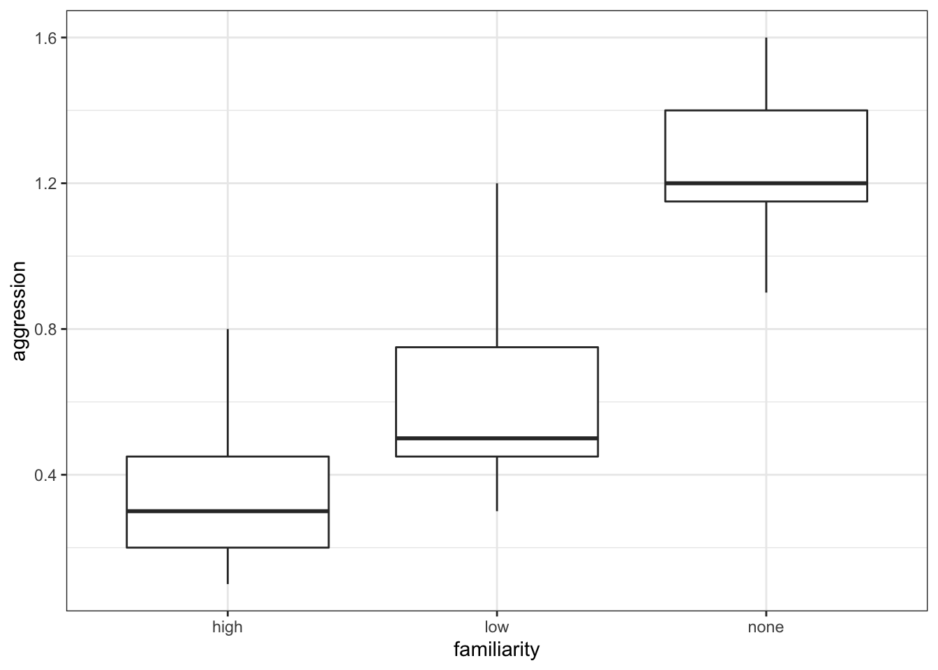

The data appear to show a very significant difference in aggression rates between the three types of familiarity. We would probably expect a reasonably significant result here.

13.6 Assumptions

To use the Kruskal-Wallis test we have to make three assumptions:

1. The parent distributions from which the samples are drawn have the same shape (if they’re normal then we should use a one-way ANOVA)
2. Each data point in the samples is independent of the others
3. The parent distributions should have the same variance

Independence we’ll ignore as usual. Similar shape is best assessed from the earlier visualisation of the data. That means that we only need to check equality of variance.

13.6.1 Equality of variance

We test for equality of variance using Levene’s test (since we can’t assume normal parent distributions which rules out Bartlett’s test).

# perform Levene's test
spidermonkey %>% 
  levene_test(aggression ~ familiarity)

## Warning in leveneTest.default(y = y, group = group, ...): group coerced to
## factor.

## # A tibble: 1 × 4
##     df1   df2 statistic     p
##   <int> <int>     <dbl> <dbl>
## 1     2    18     0.114 0.893

The relevant p-value is given in the p column (0.893). As it is quite large we see that each group do appear to have the same variance.

There is also a warning about group coerced to factor. There is no need to worry about this - Levene’s test needs to compare different groups and because aggression is encoded as a numeric value, it converts it to a categorical one before running the test.

13.7 Implement test

Perform a Kruskal-Wallis test on the data:

# implement Kruskal-Wallis test
spidermonkey %>% 
  kruskal_test(aggression ~ familiarity)

kruskal.test(aggression ~ familiarity, data = spidermonkey)

• The kruskal_test() takes the formula in the following format: variable ~ category

13.8 Interpret output and report results

This is the output that you should now see in the console window:

## # A tibble: 1 × 6
##   .y.            n statistic    df       p method        
## * <chr>      <int>     <dbl> <int>   <dbl> <chr>         
## 1 aggression    21      13.6     2 0.00112 Kruskal-Wallis

## 
##  Kruskal-Wallis rank sum test
## 
## data:  aggression by familiarity
## Kruskal-Wallis chi-squared = 13.597, df = 2, p-value = 0.001115

The p-value is given in the p column. This shows us the probability of getting samples such as ours if the null hypothesis were actually true.

Since the p-value is very small (much smaller than the standard significance level of 0.05) we can say “that it is very unlikely that these three samples came from the same parent distribution and as such we can reject our null hypothesis” and state that:

A one-way Kruskal-Wallis rank sum test showed that aggression rates between spidermonkeys depends upon the degree of familiarity between them (KW = 13.597, df = 2, p = 0.0011).

13.9 Post-hoc testing (Dunn’s test)

The equivalent of Tukey’s range test for non-normal data is Dunn’s test.

Dunn’s test is used to check for significant differences in group medians:

# perform Dunn's test
spidermonkey %>% 
  dunn_test(aggression ~ familiarity)

This will give the following output:

## # A tibble: 3 × 9
##   .y.        group1 group2    n1    n2 statistic        p    p.adj p.adj.signif
## * <chr>      <chr>  <chr>  <int> <int>     <dbl>    <dbl>    <dbl> <chr>       
## 1 aggression high   low        7     7      1.41 0.160    0.160    ns          
## 2 aggression high   none       7     7      3.66 0.000257 0.000771 ***         
## 3 aggression low    none       7     7      2.25 0.0245   0.0490   *

The dunn_test() function performs a Kruskal-Wallis test on the data, followed by a post-hoc pairwise multiple comparison.

The comparison between the pairs of groups is reported in the table at the bottom. Each row contains a single comparison. We are interested in the p and p.adj columns, which contain the the p-values that we want. This table shows that there isn’t a significant difference between the high and low groups, as the p-value (0.1598) is too high. The other two comparisons between the high familiarity and no familiarity groups and between the low and no groups are significant though.

The dunn_test() function has several arguments, of which the p.adjust.method is likely to be of interest. Here you can define which method needs to be used to account for multiple comparisons. The default is "holm". We’ll cover more about this in the chapter on Power analysis.

13.10 Exercise: Lobster weight

Exercise 13.1 Kruskal-Wallis and Dunn’s test on lobster data

Perform a Kruskal-Wallis test and do a post-hoc test on the lobster data set.

Answer

13.10.1 Hypotheses

• \(H_0\) : all medians are equal
• \(H_1\) : not all medians are equal

13.10.2 Import data, summarise and visualise

All done previously.

13.10.3 Assumptions

From before, since the data are normal enough they are definitely similar enough for a Kruskal-Wallis test and they do all have equality of variance from out assessment of the diagnostic plots. For completeness though we will look at Levene’s test

lobsters %>% 
  levene_test(weight ~ diet)

## # A tibble: 1 × 4
##     df1   df2 statistic     p
##   <int> <int>     <dbl> <dbl>
## 1     2    15   0.00280 0.997

Given that the p-value is so high, this again agrees with our previous assessment that the equality of variance assumption is well met. Rock on.

13.10.4 Kruskal-Wallis test

# implement Kruskal-Wallis test
lobsters %>% 
  kruskal_test(weight ~ diet)

## # A tibble: 1 × 6
##   .y.        n statistic    df     p method        
## * <chr>  <int>     <dbl> <int> <dbl> <chr>         
## 1 weight    18      3.26     2 0.196 Kruskal-Wallis

A Kruskal-Wallis test indicated that the median weight of juvenile lobsters did not differ significantly between diets (KW = 3.26, df = 2, p = 0.20).

13.10.5 Post-hoc Dunn’s test

Although rather unnecessary (and likely unwanted, since we don’t want to be p-hacking), because we did not detect any significant differences between diets, we can perform the non-parametric equivalent of Tukey’s range test: Dunn’s test.

# perform Dunn's test
lobsters %>% 
  dunn_test(weight ~ diet)

## # A tibble: 3 × 9
##   .y.    group1  group2     n1    n2 statistic      p p.adj p.adj.signif
## * <chr>  <chr>   <chr>   <int> <int>     <dbl>  <dbl> <dbl> <chr>       
## 1 weight Flakes  Mussels     6     7     1.79  0.0738 0.221 ns          
## 2 weight Flakes  Pellets     6     5     0.670 0.503  0.629 ns          
## 3 weight Mussels Pellets     7     5    -1.01  0.315  0.629 ns

We can see that none of the comparisons are significant, either based on the uncorrected p-values (p) or the p-values adjusted for multiple comparisons (p.adj). This is consistent with what we found previously.

13.11 Key points

• We use Kruskal-Wallis test to see if there is a difference in medians between multiple continuous variables
• In R we first define a linear model with lm(), using the format response ~ predictor
• Next, we perform a Kruskal-Wallis test on the linear model with kruskal_test()
• We assume parent distributions have the same shape; each data point is independent and the parent distributions have the same variance
• We test for equality of variance using levene_test()
• Post-hoc testing to check for significant differences in the group medians is done with dunn_test()