9 Wilcoxon signed-rank test

A Wilcoxon signed-rank test is an alternative to a paired t-test. It does not require that the data are drawn from normal distributions, but it does require that the distribution of the differences is symmetric. We’re effectively testing to see if the median of the differences between the two samples differs significantly from zero.

9.1 Section commands

There are no new commands in this section.

9.2 Data and hypotheses

Using the cortisol dataset from before we form the following null and alternative hypotheses:

• \(H_0\): The median of the difference in cortisol levels between the two groups is 0 \((\mu M = \mu E)\)
• \(H_1\): The median of the difference in cortisol levels between the two groups is not 0 \((\mu M \neq \mu E)\)

We use a two-tailed Wilcoxon signed-rank test to see if we can reject the null hypothesis.

9.3 Summarise and visualise

Already implemented previously.

9.4 Assumptions

These have been checked previously.

9.5 Implement test

Perform a two-tailed, Wilcoxon signed-rank test:

# perform the test
cortisol %>% 
  wilcox_test(cortisol ~ time,
              alternative = "two.sided",
              paired = TRUE)

• The first argument gives the formula
• The second argument gives the type of alternative hypothesis and must be one of two.sided, greater or less
• The third argument says that the data are paired

9.6 Interpret output and report results

## # A tibble: 1 × 7
##   .y.      group1  group2     n1    n2 statistic        p
## * <chr>    <chr>   <chr>   <int> <int>     <dbl>    <dbl>
## 1 cortisol evening morning    20    20        13 0.000168

The p-value is given in the p column (p-value = 0.000168). Given that this is less than 0.05 we can still reject the null hypothesis.

A two-tailed, Wilcoxon signed-rank test indicated that the median cortisol level in adult females differed significantly between the morning (320.5 nmol/l) and the evening (188.9 nmol/l) (V = 197, p = 0.00017).

9.7 Exercise: Deer legs

Exercise 9.1 Deer legs

Using the following data, test the null hypothesis that the fore and hind legs of deer are the same length.

## # A tibble: 10 × 2
##    hindleg foreleg
##      <dbl>   <dbl>
##  1     142     138
##  2     140     136
##  3     144     147
##  4     144     139
##  5     142     143
##  6     146     141
##  7     149     143
##  8     150     145
##  9     142     136
## 10     148     146

Do these results provide any evidence to suggest that fore- and hind-leg length differ in deer?

1. Write down the null and alternative hypotheses
2. Choose a tidy representation for the data and create a csv file (I’ll stop asking you to do this from now on…)
3. Import the data into R
4. Summarise and visualise the data
5. Check your assumptions (normality and variance) using appropriate tests
6. Discuss with your (virtual) neighbour which test is most appropriate?
7. Perform the test
8. Write down a sentence that summarises the results that you have found

Answer

9.7.1 Hypotheses

\(H_0\) : foreleg average (mean or median) \(=\) hindleg average (mean or median)

\(H_1\) : foreleg average \(\neq\) hindleg average

9.7.2 Import data, summarise and visualise

First of all, we need to get the data into a tidy format (every variable is a column, each observation is a row). Doing this in Excel, and adding a ID gives us:

# load the data
deer <- read_csv("data/examples/cs1-deer.csv")

# have a look
deer

## # A tibble: 20 × 3
##       id leg     length
##    <dbl> <chr>    <dbl>
##  1     1 hindleg    142
##  2     2 hindleg    140
##  3     3 hindleg    144
##  4     4 hindleg    144
##  5     5 hindleg    142
##  6     6 hindleg    146
##  7     7 hindleg    149
##  8     8 hindleg    150
##  9     9 hindleg    142
## 10    10 hindleg    148
## 11     1 foreleg    138
## 12     2 foreleg    136
## 13     3 foreleg    147
## 14     4 foreleg    139
## 15     5 foreleg    143
## 16     6 foreleg    141
## 17     7 foreleg    143
## 18     8 foreleg    145
## 19     9 foreleg    136
## 20    10 foreleg    146

The ordering of the data is important here; the first hindleg row corresponds to the first foreleg row, the second to the second and so on. To indicate this we use an id column, where each observation has a unique ID.

Let’s look at the data and see what we can see.

# summarise the data
deer %>% 
  select(-id) %>% 
  get_summary_stats(type = "common")

## # A tibble: 1 × 10
##   variable     n   min   max median   iqr  mean    sd    se    ci
##   <chr>    <dbl> <dbl> <dbl>  <dbl> <dbl> <dbl> <dbl> <dbl> <dbl>
## 1 length      20   136   150    143  5.25  143.  4.01 0.896  1.88

# or even summarise by leg type
deer %>% 
  select(-id) %>% 
  group_by(leg) %>% 
  get_summary_stats(type = "common")

## # A tibble: 2 × 11
##   leg     variable     n   min   max median   iqr  mean    sd    se    ci
##   <chr>   <chr>    <dbl> <dbl> <dbl>  <dbl> <dbl> <dbl> <dbl> <dbl> <dbl>
## 1 foreleg length      10   136   147    142  6.25  141.  4.03  1.27  2.88
## 2 hindleg length      10   140   150    144  5.5   145.  3.40  1.08  2.43

# we can also visualise the data
deer %>% 
  ggplot(aes(x = leg, y = length)) +
  geom_boxplot()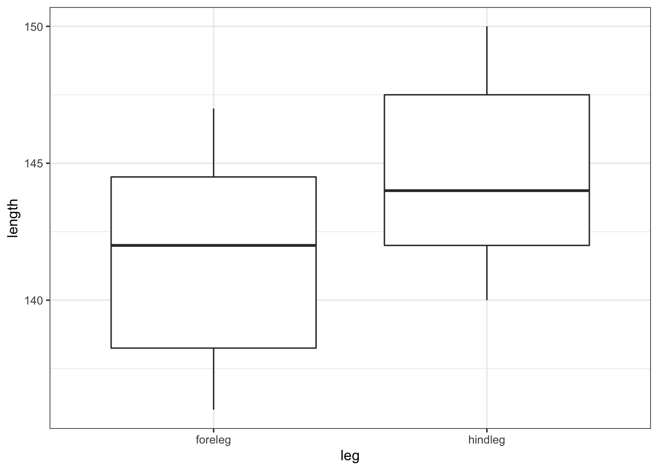

All of this suggests that there might be a difference between the legs, with hindlegs being longer than forelegs. However, this representation obscures the fact that we have paired data. What we really need to look at is the difference in leg length for each deer and the data by observation:

# create a data set that contains the difference in leg length
leg_diff <- deer %>% 
  pivot_wider(names_from = leg, values_from = length) %>% 
  mutate(leg_diff = hindleg - foreleg)

# plot the difference in leg length
leg_diff %>% 
  ggplot(aes(y = leg_diff)) +
  geom_boxplot()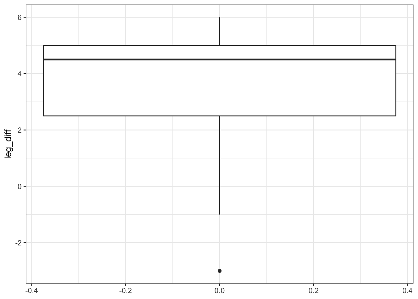

Additionally, we can also plot the data by observation:

# plot the data by observation
deer %>% 
  ggplot(aes(x = leg, y = length, group = id)) +
  geom_point() +
  geom_line()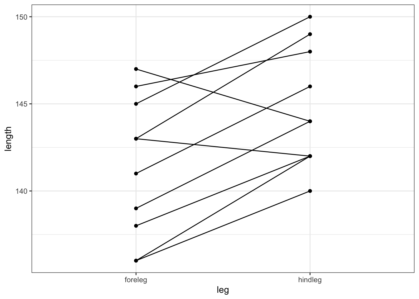

This gives us a much clearer picture. It looks as though the hindlegs are about 4 cm longer than the forelegs, on average. It also suggests that our leg differences might not be normally distributed (the data look a bit skewed in the boxplot).

9.7.3 Assumptions

We need to consider the distribution of the difference in leg lengths rather than the individual distributions.

# perform Shapiro-Wilk test on leg differences
leg_diff %>% 
  shapiro_test(leg_diff)

## # A tibble: 1 × 3
##   variable statistic      p
##   <chr>        <dbl>  <dbl>
## 1 leg_diff     0.814 0.0212

# and create a Q-Q plot
lm_leg_diff <- lm(leg_diff ~ 1,
                  data = leg_diff)


lm_leg_diff %>% 
  resid_panel(plots = "qq")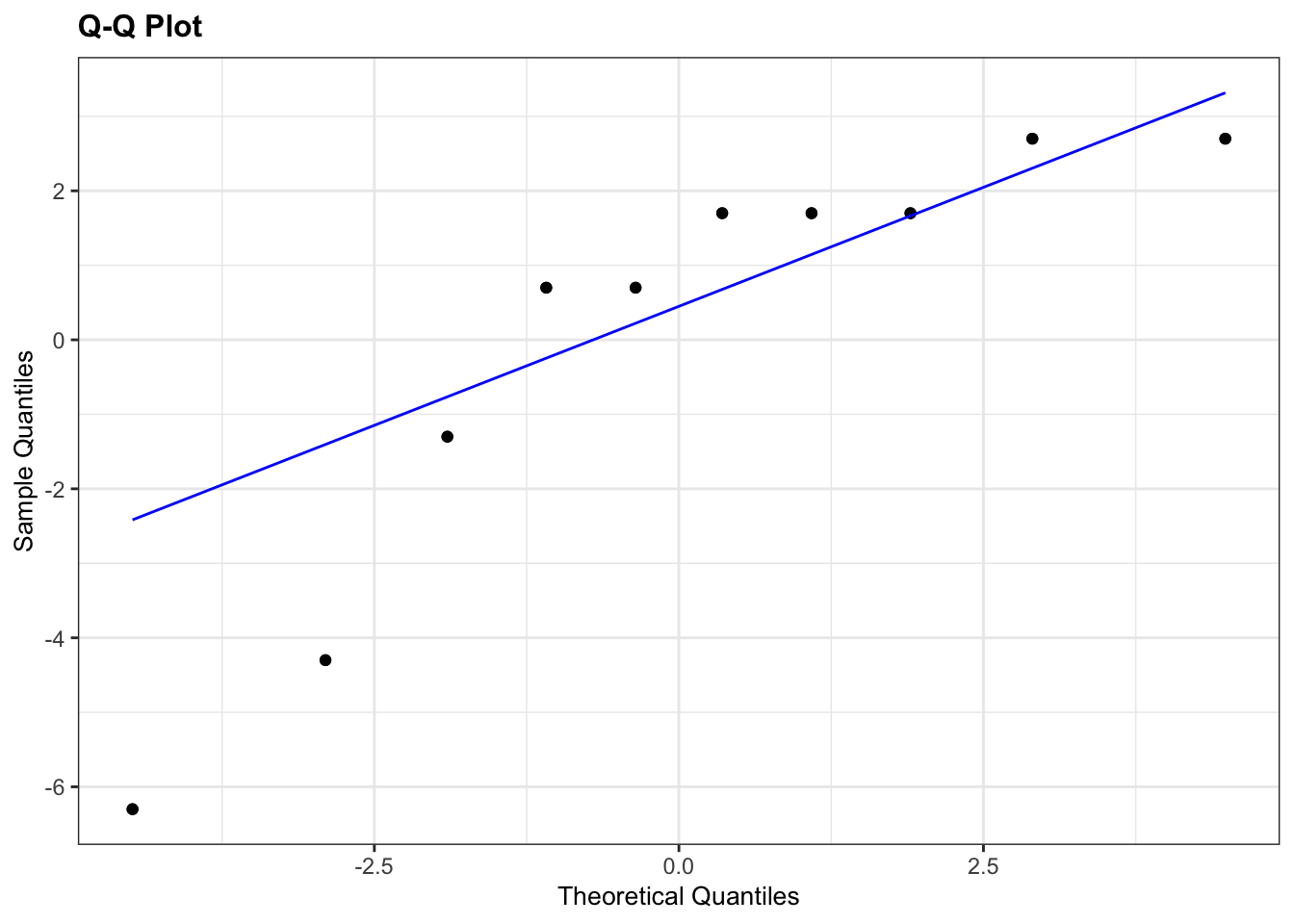

Both our Shapiro-Wilk test and our Q-Q plot suggest that the difference data aren’t normally distributed, which rules out a paired t-test. We should therefore consider a paired Wilcoxon test next. Remember that this test requires that the distribution of differences be symmetric, whereas our box-plot from before suggested that the data were very much skewed.

9.7.4 Conclusions

So, frustratingly, neither of our tests are appropriate for this dataset. The differences in foreleg and hindleg lengths are neither normal enough for a paired t-test nor are they symmetric enough for a Wilcoxon test and we don’t have enough data to just use the t-test (we’d need more than 30 points or so). So what do we do in this situation? Well the answer is that there aren’t actually any traditional statistical tests that are valid for this dataset as it stands!

There are two options available to someone:

1. try transforming the raw data (take logs, square root, reciprocals) and hope that one of them leads to a modified dataset that satisfies the assumptions of one of the tests we’ve covered, or
2. use a permutation test approach (which would work but is beyond the scope of this course).

The reason I included this example in the first practical is purely to illustrate how a very simple dataset with an apparently clear message (leg lengths differ within deer) can be intractable. You don’t need to have very complex datasets before you go beyond the capabilities of classical statistics.

As Jeremy Clarkson would put it:

And on that bombshell, it’s time to end. Goodnight!

9.8 Key points

• We use two-sample tests to see if two samples of continuous data come from the same parent distribution
• This essentially boils down to testing if the mean or median differs between the two samples
• There are 5 key two-sample tests: Student’s t-test, Welch’s t-test, Mann-Whitney U test, paired t-test and Wilcoxon signed-rank test
• Which one you use depends on normality of the distribution, sample size, paired or unpaired data and variance of the samples
• Parametric tests are used if the data are normally distributed or the sample size is large
• Non-parametric tests are used if the data are not normally distributed and the sample size is small
• Equality of variance then determines which test is appropriate
• You can ask yourself 3 questions to determine the test:
  1. is my data paired?
  2. do I need a parametric or non-parametric test
  3. can I assume equality of variance?